Income-Expenditure Model

The income-expenditure model of GDP, also called the Keynesian model since it was pioneered by Keynes, is a model that asserts that the real GDP at equilibrium is entirely determined by the desired level of aggregate expenditure on domestically-produced final goods & services by all people, households, firms, foreigners and the government. This is called the planned aggregate expenditure, $PAE$.

Basically, the income-expenditure model expects a country’s GDP to be equal to the planned aggregate expenditure, ie. the equilibrium condition is:

$$Y_{\text{equilibrium}}=PAE=C+I^P+G+NX.$$

See the expenditure approach of calculating GDP.

• $I^P$ is the planned investment as opposed to actual investment $I$. They differ in value because of unplanned changes to firms’ inventories, given by: $I=I^P+\Delta {\text{Inv}}_{\text{unplanned}}$.
• Unplanned inventory — the difference between the actual expenditure and the planned expenditure.

Assumptions

A key assumption of the income-expenditure model is that prices of goods & services are ‘fixed’ (or ‘sticky’). It assumes that firms will not change the prices of their goods & services in response to a change in demand for them in the short-run. Instead, they’ll respond by adjusting their level of production.

Note: this is a fair assumption since firms cannot know whether it’s reasonable to change costs so quickly, due to menu costs. Why? Suppose you’re a cafe owner. When there’s a sudden influx of demand, you would probably crank up the level of production rather than increasing the cost of coffee. Eventually in the long-run, if you see that this demand persists then you’d increase prices.

Disequilibrium

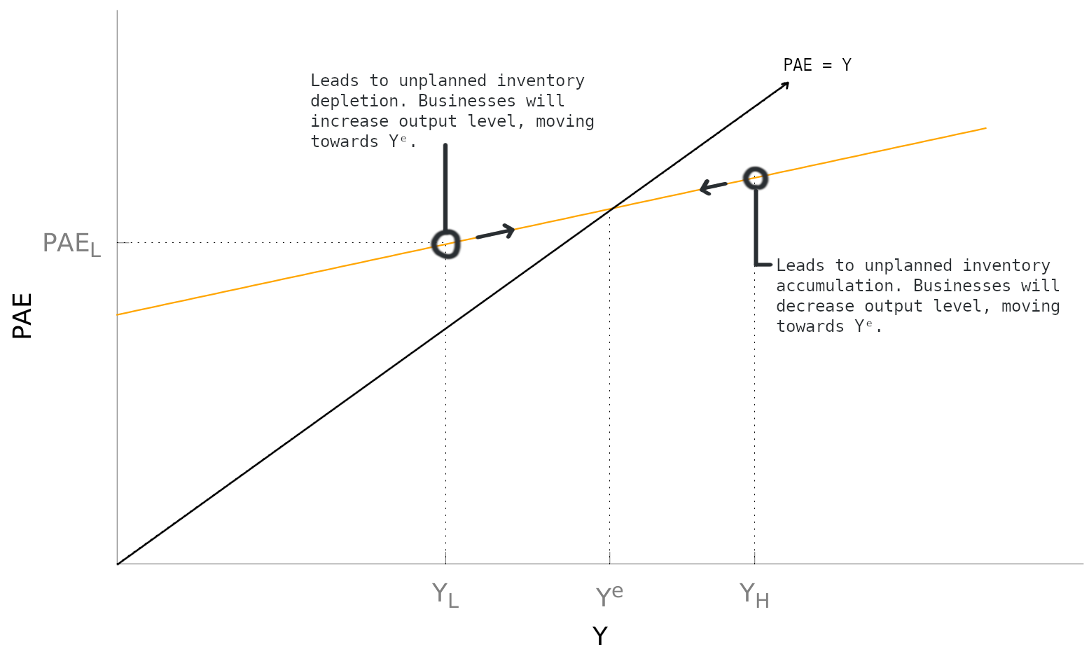
The business sector can produce at a level greater than or less than the $PAE$, in which case the economy would be in disequilibrium.

If $Y>PAE$, businesses have produced more goods & services than all sectors were willing to purchase. This leads to an unplanned increase in their inventories, and will prompt businesses to reduce their production levels accordingly, causing GDP to fall until the equilibrium condition $Y=PAE$ is satisfied.

Likewise, if $Y<PAE$, then businesses have produced less than what all sectors were willing to purchase, unexpectedly depleting their inventories. They’ll ramp up production, until $Y=PAE$.

Graphically, it looks like this:

Consumption Function

In the income-expenditure model, we model household consumption, $C$, using the Keynesian consumption function:

$$C=C_0+c\underset{\text{Disp. income}}{\underbrace{(Y-T)}}.$$

• $C_0$ is an exogenous variable representing how much households will spend on consumption when their disposable income is $0$. An assumption here is that $C_0>0$.
• $c$ is the marginal propensity to consume, $MPC$. A key assumption is that $0<c<1$. In the above consumption function, if your income were to rise by \1$,yourmarginalpropensitytoconsumeishowmuchofthat$$1$ you will spend on consumption instead of save.
  • Note: we also call $1-c$ the marginal propensity to consume.
• Average propensity to consume, $APC$, is the percentage of income that is spent rather than saved. It can be obtained as $APC=\frac{C}{Y-T}=\frac{C_0}{Y-T}+c$.

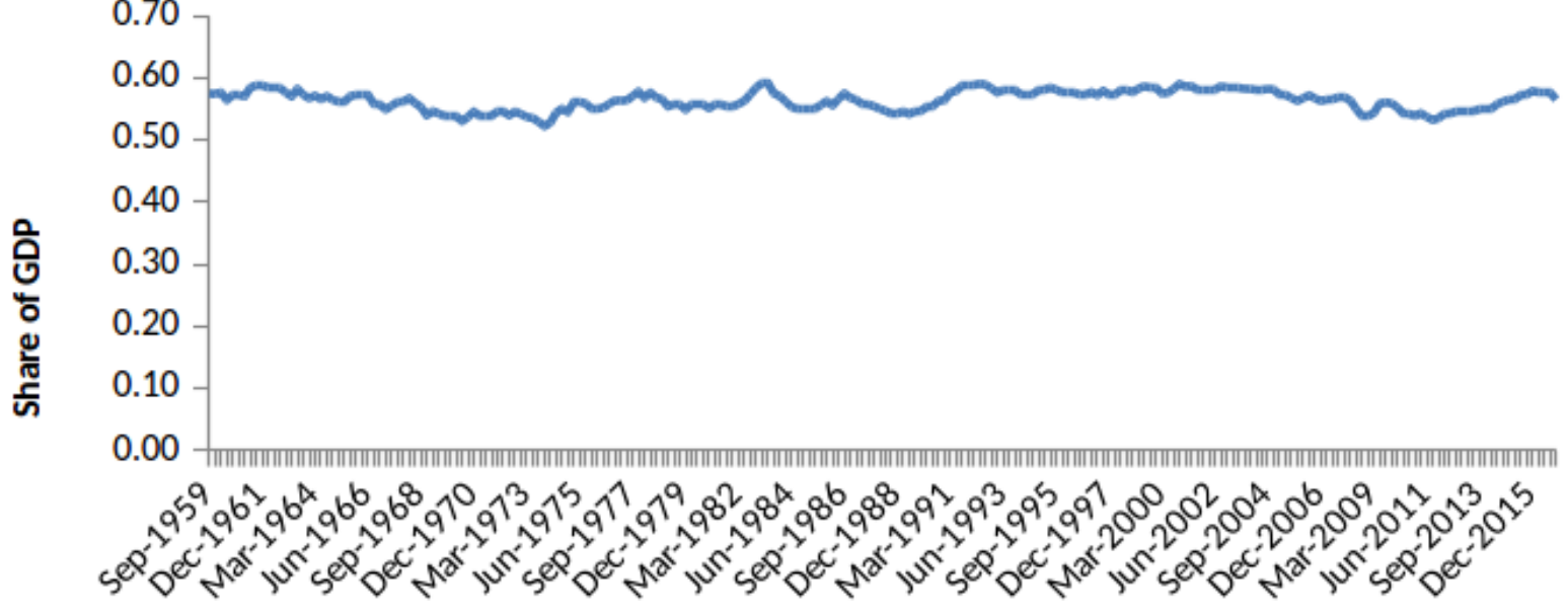
Household consumption is a stable and major contributor to GDP, sitting at around $\approx 60\%$ in Australia.

2-Sector Economy

Consider an economy that only consists of households and businesses. In this case, we’d have $Y=C+I^P$. At equilibrium, we can see that:

$$\begin{array}{rl}{Y}_{\text{Equilibrium}}& =PAE=C+I_0\\ & =C_0+cY+I_0\\ & =\frac{1}{1-c}(C_0+I_0),\end{array}\text{\hspace{1em}(1)}$$

where $\frac{1}{1-c}$ is called the multiplier.

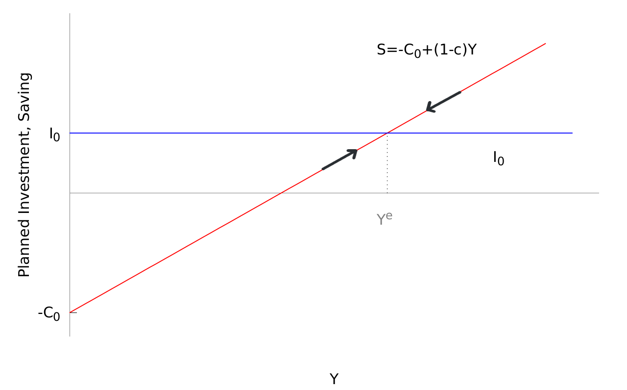
Savings and Investment At equilibrium, the savings is equal to the planned investment:

$$\begin{array}{rl}Y& =PAE\\ & =C+I^P\\ Y-C& =I^P\\ S& =I^P.\end{array}$$

From the consumption function, we can express a saving function,

$$\begin{array}{rl}S& =Y-C\\ & =Y-(C_0+cY)\\ & =-C_0+(1-c)Y,\end{array}$$

Opening the 2-Sector Economy Now let’s the consider the economy that includes imports/exports. We have $PAE=C+I^P+X-M$. Assuming that the imports scales linearly with GDP: $M=mY$, where $0<m<c$ is the marginal propensity to import, we can derive:

$$\begin{array}{rl}{Y}_{\text{Equilibrium}}& =PAE=C+I^P+X-M\\ & =C_0+cY+I_0+X_0-mY\\ & =\frac{1}{1-(c-m)}(C_0+I_0+X_0).\end{array}\text{\hspace{1em}(2)}$$

Comparing this result with $(1)$, we see that opening the economy makes the multiplier smaller.

Paradox of Thrift

The ‘paradox of thrift’ is a paradox where an increase in exogenous household saving, $C_0$, which shifts the aggregate saving function up, does not actually increase the amount of real savings. This is because a collective effort of every household to save simply causes the production levels to drop, meaning a reduction in equilibrium GDP and the effects of saving are nullified as shown:

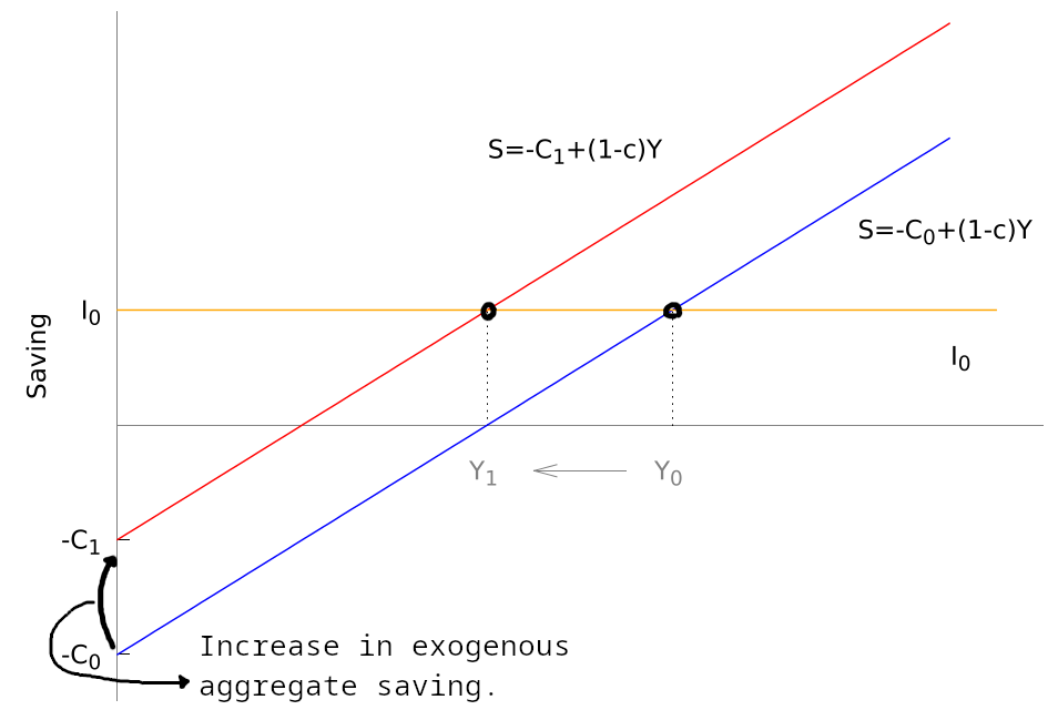
The Paradox of Thrift suggests that while it may be wise for an individual to save money when income is low and job prospects are precarious, it could be collectively disastrous if everyone is thrifty together.

The paradox of thrift is an example of a fallacy of composition. An example of the fallacy of composition: when you stand up amongst a crowd to get a better view of something, it only works when a few people do it. When everyone does it, then the gains from standing up are nullified. At that point, it would be equivalent to if everyone remained seated.