Aggregate Supply and Demand

The income-expenditure model aims to determine the short-run real GDP. The aggregate supply and demand model aims to determine the real GDP in both the short-run and long-run.

Note that the aggregate demand and aggregate supply curves are different in meaning fundamentally to the marginal benefit and marginal cost curves in microeconomic contexts.

Aggregate Demand (AD)

Recall that the planned aggregate expenditure in a 4-sector economy is given as $PAE=C+I^P+G+X-M$.

One core assumption is that a rise in $r$ will tend to reduce consumption and planned investment. We can assume they are affected in the following way:

• $C=C_0+c(Y-T)-\alpha r$, where $\alpha >0$.
• $I^P=I_0-\beta r$, where $\beta >0$.

Plugging these in and solving for the equilibrium real GDP, we get:

$$\begin{array}{rl}{Y}_{\text{equilibrium}}& =PAE=[C_0+c(Y-T)-\alpha r]+[I_0-\beta r]+G_0+X_0-mY\\ & =\frac{1}{1-c(1-t)+m}\left(\right(C_0-c{T}_0+I_0+G_0+X_0)-r(\alpha +\beta )).\end{array}$$

Now we’ve made $Y_{\text{equilibrium}}$ a function of $r$, we have a simple model for predicting the effects of monetary policy on real GDP.

To express $Y_{\text{equilibrium}}$ as a function of $\pi$, we can assume that the central bank will use the simple policy rule reaction function which tells them to increase the real interest rate in response to an increase in inflation rate. With this assumption, we can relate the real interest rate with the inflation rate, $r=r_0+\gamma \pi$ and express $Y_{\text{equilibrium}}$ as a function of $\pi$:

$$\begin{array}{rl}{Y}_{\text{equilibrium}}& =\frac{1}{1-c(1-t)+m}\left(\right(C_0-c{T}_0+I_0+G_0+X_0)-r(\alpha +\beta )),\\ & =\frac{1}{1-c(1-t)+m}\left(\right(C_0-c{T}_0+I_0+G_0+X_0)-(r_0+\gamma \pi )(\alpha +\beta )),\\ & \\ \text{Supposing }k& =\frac{1}{1-c(1-t)+m},\\ Y_{\text{equilibrium}}& =k(C_0-c{T}_0+I_0+G_0+X_0-r_0(\alpha +\beta ))-k\gamma (\alpha +\beta )\pi .\\ & \end{array}$$

Supposing $A_0=k\underset{\text{Exogenous variables}}{\underbrace{(C_0-c{T}_0+I_0+G_0+X_0-r_0(\alpha +\beta ))}}$, we now have an equation representing the aggregate demand curve: $Y_{\text{equilibrium}}=A_0-k\gamma (\alpha +\beta )\pi ,$ which relates the real GDP to the inflation rate. Although the AD curve links the real GDP and inflation, it does not determine them. That’s where we need the aggregate supply curve.

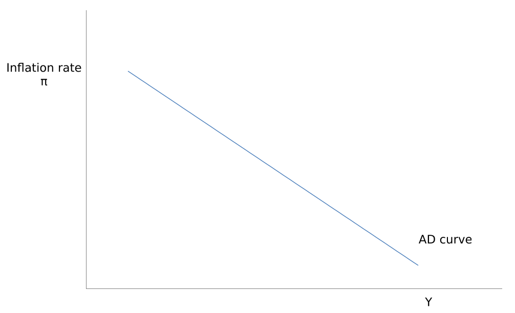
Changes to the exogenous variables in the constant $A_0=k(C_0-c{T}_0+I_0+G_0+X_0-r_0(\alpha +\beta ))$ will cause shifts in the AD curve, often called AD shocks.

Note that when productivity is low, ie. real GDP is low, prices are high.

Aggregate Supply (AS)

In the income-expenditure model, we assumed that the prices would stay fixed in the short run. In the aggregate supply and demand model, we assume that the business will choose the new prices, thereby setting the actual inflation rate, based on 3 factors:

1. The expected inflation rate.

   Rational expectations hypothesis — asserts that people always factor in all relevant information, producing the best theoretical possible forecast on what the future inflation rate will be. The actual and expected value differ by a completely unpredictable margin, $\omega$: ${\pi }_{\text{actual}}={\pi }_{\text{expected}}+\omega$

   Adaptive expectations hypothesis — asserts that people will use historical data only in their prediction of the future inflation rate, ie. that ${\pi }_{\text{actual}}={\pi }_{\text{prev}}$, which makes the AS curve a simple horizontal line:

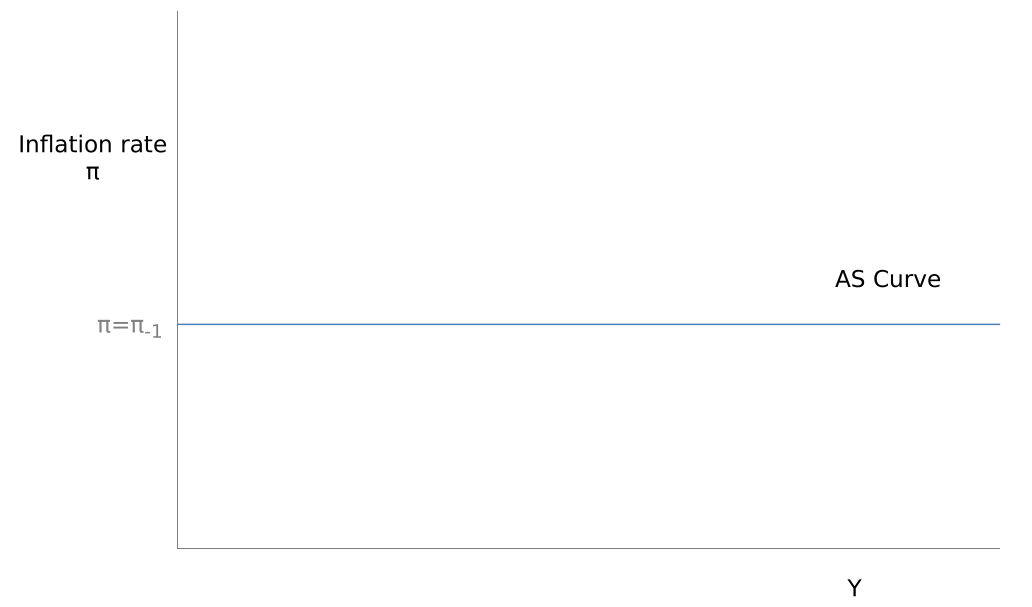
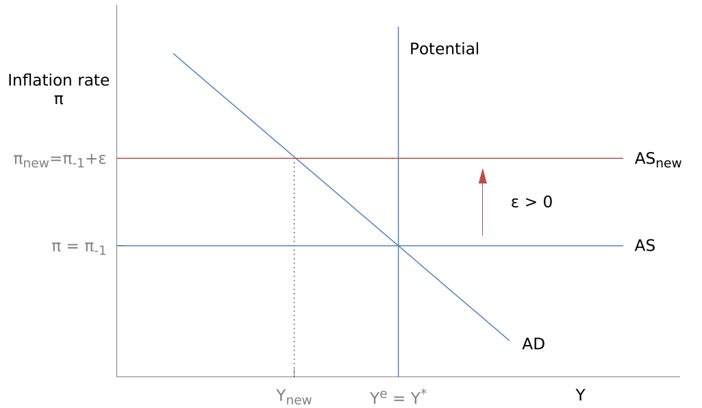
   Inflation shocks are when there are changes to the inflation rate. Events that might cause inflation shocks include changes in commodity prices and foreign exchange rates. Factoring in inflation shocks, we’d have ${\pi }_{\text{actual}}={\pi }_{\text{prev}}+ϵ$, where $ϵ$ is the size of the inflation shock. Note that inflation shocks, although temporary in nature, cause permanent effects to the inflation rate since the adaptive expectations hypothesis asserts that the next period’s inflation rate retains the previous period’s inflation rate.

2. Shifts in the aggregate demand curve which impact the business’ production costs.

3. Size of the output gap.

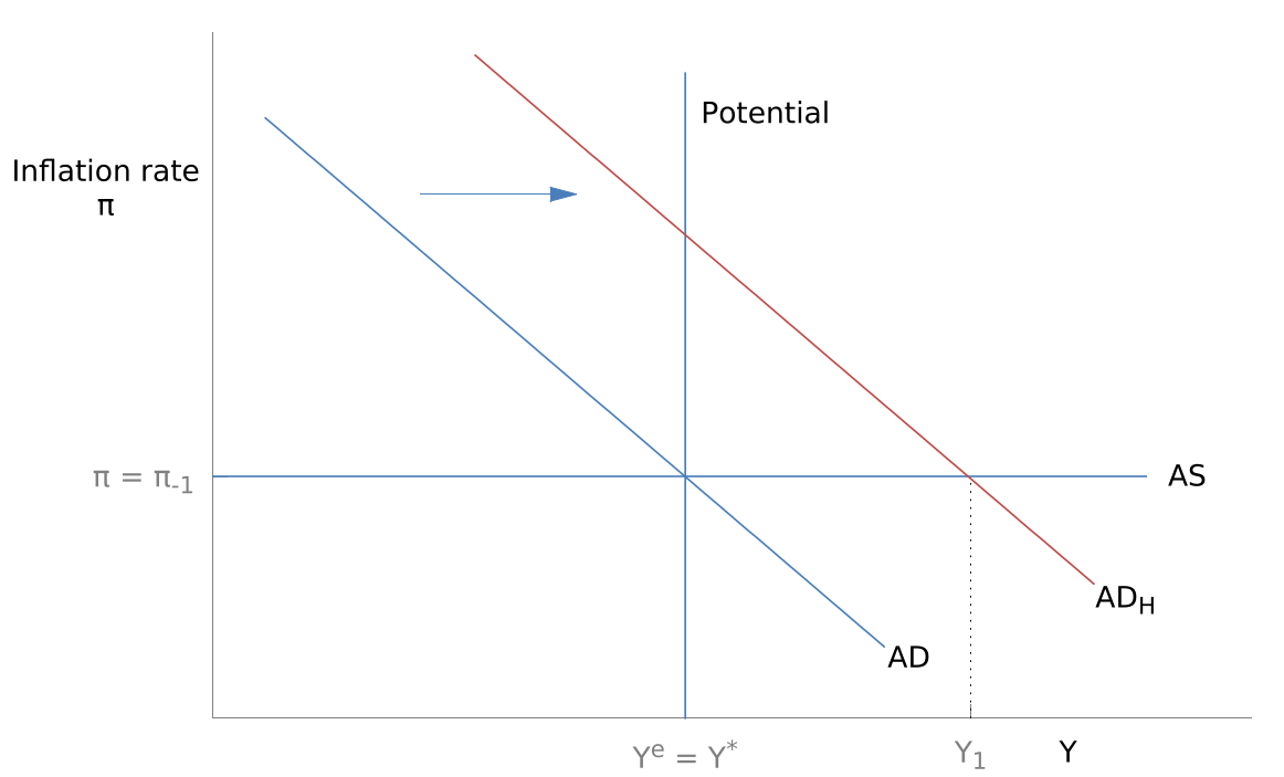
   When there exists a short-run expansionary output gap like below for example, businesses will initially ramp up production levels to meet increased demand, but over time they’ll experience increased production costs and inflate their prices. When all businesses behave this way, then in aggregate, it’ll cause inflation to increase and close the output gap.

   

Applications

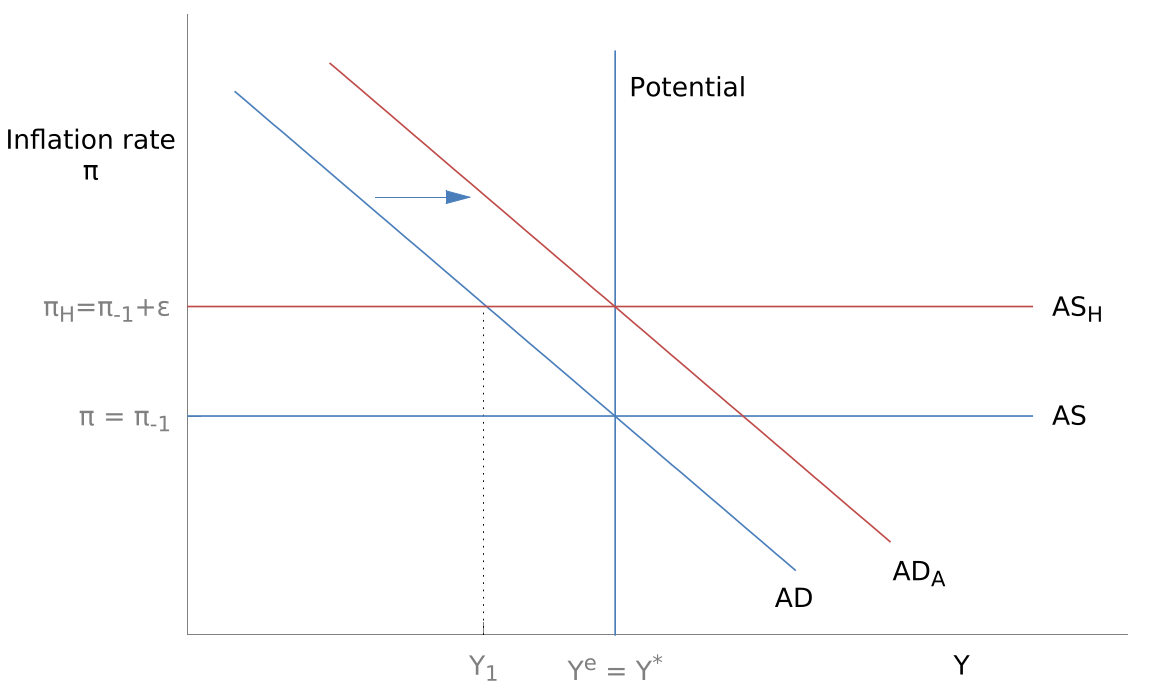
If households were to collectively become more optimistic about wage growth and were to start consuming more, then this could cause an increase in $C_0$, causing an AD shock that shifts the curve up, causing the real GDP to increase but with inflation staying constant in the short-run:

Progressing towards the long-run, the AS curve will shift up to close the expansionary output gap.

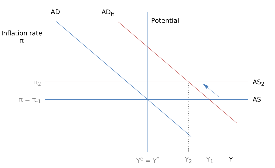
Inflation will keep increasing until $Y_{\text{equilibrium}}=Y^{\ast }$.

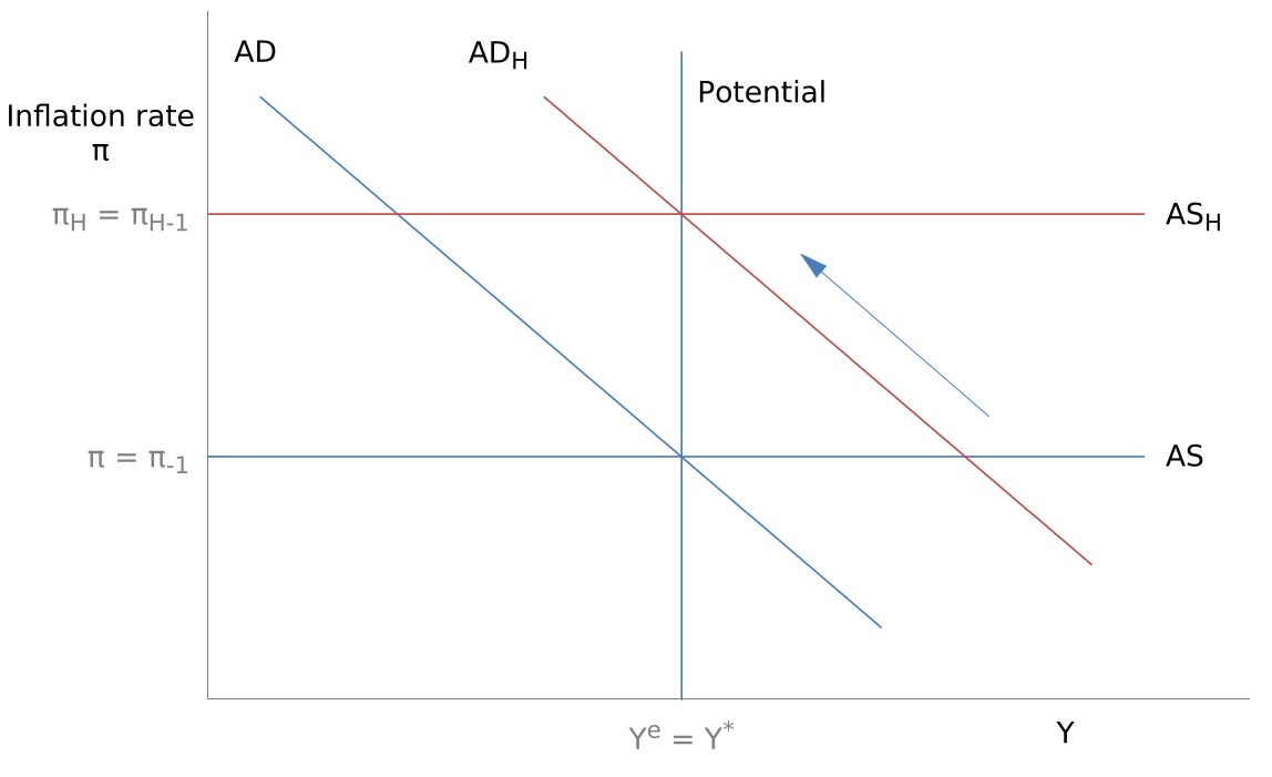
When an inflation shock happens and shifts the AS curve upwards, it’ll be the case that in the long run, the inflation rate will drop to the same level prior to the shock.

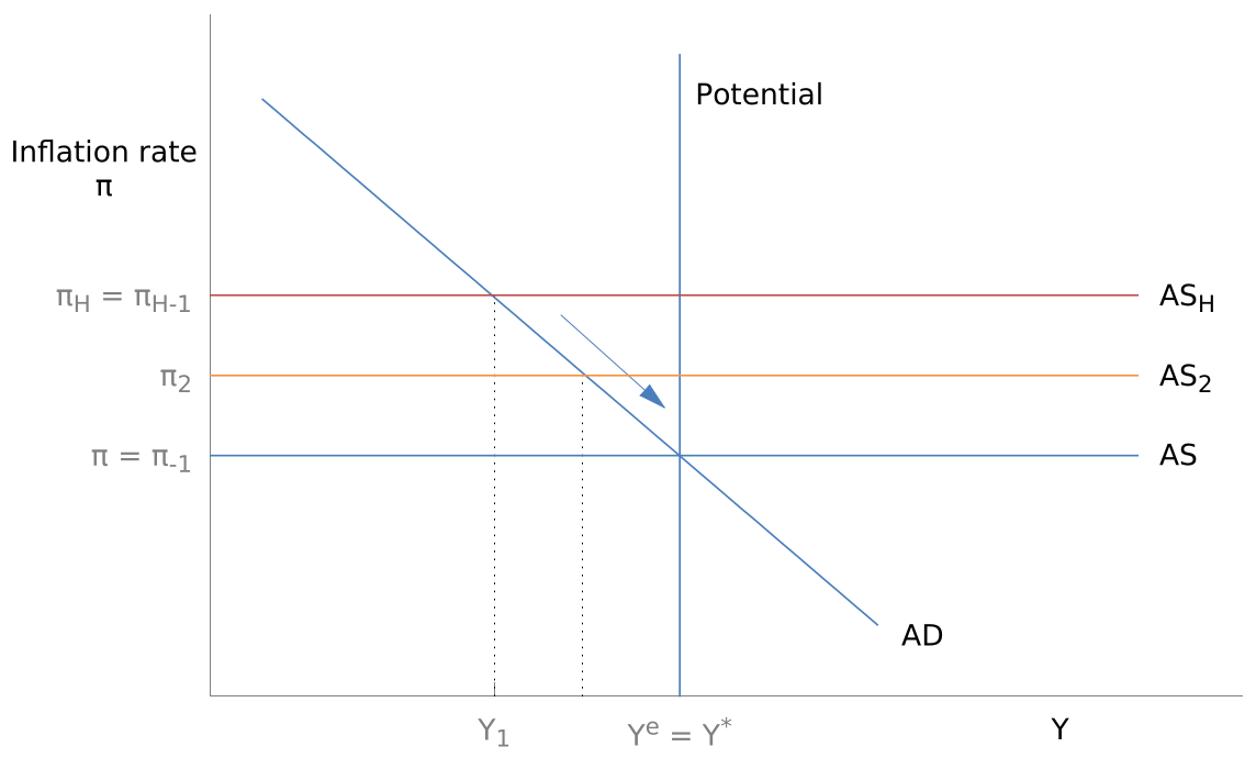
Notice how the economy ‘self-corrects’ in the long run. Does this mean that fiscal and monetary policy are unnecesssary? No, because they can accelerate the self-correction and minimise the negative effects of AD shocks and inflation shocks.

Note that in the above example, the government and central bank could choose to ‘accommodate’ the inflation shock by implement tax cuts (or some other policy) to shift up the AD curve and meet the higher inflation value. Doing this will mean that the contractionary gap is closed quicker, but the higher inflation will tend to persist instead of being temporary. If they don’t want higher inflation to persist (in order to ensure they meet an inflation target), then they can simply do nothing and let the self-correction proceed.